Inhibitory interactions between progenitor cells bias the distribution of NSC activation events

(A–A’’') Confocal dorsal views of a whole-mount adult telencephalon showing the germinal layer of the pallium in a 3mpf Tg(gfap:GFP) fish immunostained for GFP (green, NSCs), PCNA (magenta, proliferating cells), and Gfap (Zrf1 antibody, cyan). Anterior left, pallial subdivisions (Dl: lateral, Dm: medial, Da: anterior) indicated by dotted lines.

(A and A’) Dorsal (apical) view and high magnification of the NSC layer, showing merged and single channels (color-coded). Arrowheads: purple to aNSCs, orange to aNPs. aNSCs are GFP⁺,Gfap⁺, aNPs are negative for both markers.

(A’’ and A’’’) Examples of aNSCs with a process (red arrows) visible using the GFP or the Zrf1 markers, respectively (left and right panels: different backgrounds to ease observation).

(B–B’’) Similar sample stained for GFP (green, NSCs) and PCNA (magenta, proliferating cells).

(B and B’) Merged and single-channel views (color-coded).

(B’’) Close-up in Dm showing progenitor cell states (merged image, individual channels and segmentation): quiescent NSCs (qNSCs; GFP⁺ only; green), activated NSCs (aNSCs; GFP⁺,PCNA⁺; magenta), and proliferating neural progenitors (aNPs; PCNA⁺ only; orange) (see also Figures S1A–A”).

(A, B, and B') Stitches of 4 tiles with 10% overlap.

(C) Main pallial NSC lineage (arrows: lineage transitions).

(D) Proportions of qNSCs, aNSCs, and aNPs relative to each other in Dm (see also Figures S1B–B’’’).

(E) Besag’s L function assessing spatial correlations for the same fish between aNSCs (left) and between aNSCs and aNPs (right) (aNSCs include pre-division aNSCs—singlets—and immediately post-division NSCs—doublets, scheme on left). L_(obs)(r) (red line): experimental value, L_{(H0, mean)}(r) (black dotted line): mean under the random labeling null hypothesis (the state of any cell is independent of other cells and of its position), r: mean cell diameter in this brain (r = 0: cell of reference, r = 1: immediate neighbor), gray regions: 95% confidence envelopes. High magnification shows significant dispersion (see also Figures S2A–S2E).

(F) Range and strength of this interaction determined with functions g (left) and M (right). Green bar: 95^th centile of the distance to the furthest direct neighbor of aNPs.

Scale: (A), (B), and (B’) 100 μm; (A’) 10 μm; (A’’), (A’’’) 7 μm; (B’’) 30 μm.

The lower incidence of activated NSCs close to aNPs is Notch signaling dependent

(A) Confocal whole-mount view of the pallial germinal layer in a 3mpf Tg(gfap:tdTomato);Tg(delta:GFP) fish stained for tdTomato (NSCs, green), GFP (deltaA expression, cyan) and PCNA (magenta) (DeltaA channel only). Anterior, left. (A) Stitch of 4 tiles with 15% overlap.

(B–B’’’) Close-ups in Dm, all channels. Arrowheads: magenta, aNSC; orange, aNP; expressing deltaA.

(C–C’’) Percentages of aNSCs (all, pre-, or post-division) among all NSCs (C and C”) or aNSCs (C’) upon 24-h LY treatment (DMSO: control). ns, non-significant; unpaired t test (see also Figures S2F, S3A–S3C, and S4A–S4B’’).

(D–D”) Number (D and D’) and proportion (D’’) of aNSCs, in total (D) or touching aNPs upon 24-h LY treatment (DMSO: control) (D’’, p = 0.002, t test) (see also Figure S3C).

(E) Spatial distribution (Besag’s L function) of aNSC singlets relative to each other (left) and to aNPs (right) upon 24-h LY treatment (DMSO: control). L_(obs)(r) (red lines): experimental values; L_(H0,mean)(r) (black dotted lines): means under the random labeling null hypothesis; r: mean NSC diameter; gray regions: 95% confidence envelopes. Arrowheads: red, aNP inhibitory effect; black, disappearance upon LY (see also Figures S4C–S4F).

Scale: (A) 40 μm, (B)–(B’’’) 20 μm.

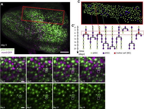
Intravital imaging resolves adult NSC lineage trees in time and space

(A) Whole pallial hemisphere imaged intravitally in a 3mpf casper;Tg(gfap:dTomato);Tg(mcm5:GFP) fish (named Mimi) (anterior left, tile of 4 images with 10% overlap, taken at day 3 from a 35-day session of recordings every 3–4 days, 8 time points). Colors of the live reporters were adjusted (green: NSCs, magenta: proliferating cells).

(B) Close-ups from the same video showing an asymmetric NSC division (dotted circles) between days 3 and 9: 1 daughter differentiates over the next 7 days (bottom dotted circle, loss of the gfap:dTomato signal). White asterisks: random qNSCs close to the division, used for alignment.

(C and C’) Segmentation and NSC tracking over 23 days in Dm in Mimi. (C) Segmentation of ~390 cells per time point (area boxed in A, at day 6). (C’) Example of dividing tracks, with cell states (color-coded) and the spatial position of each tree (see also Figure S5A). Scale bars: (A), 100 μm; (B), 20 μm.

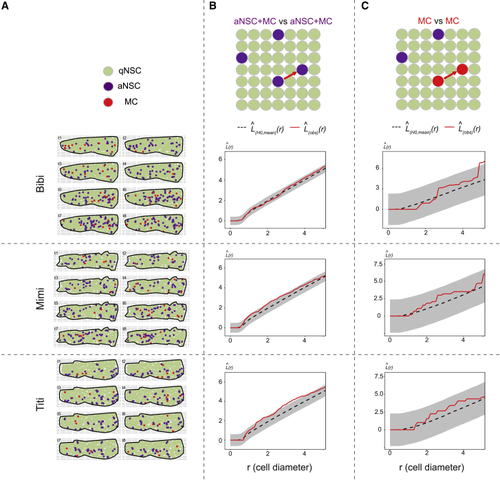
Static spatial analysis of NSC activation from dynamic datasets

(A) Dm surfaces segmented for the 3 fish analyzed (Bibi, Mimi, Titi) at all time points, cell states color-coded (see also Figures S5B–S5F).

(B and C) L functions comparing the positions of aNSCs+MCs with one another (B), and MCs with one another (C) for each fish (see also Figures S5A–S5F). L_(obs)(r) (red lines): experimental values, L functions for all time points pooled using a weighted average; L_{(H0, mean)}(r) (black dotted lines): means under the random labeling null hypothesis; r: mean NSC diameter for each Dm surface; gray regions: 95% confidence envelopes. Pooled p > 0.01 in (B) and (C) for the [0–2] (r) interval.

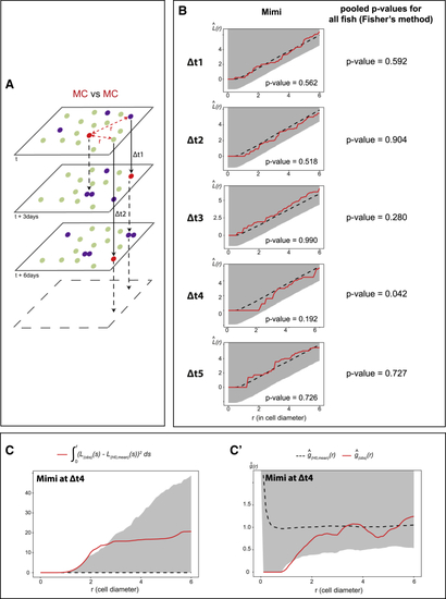
NSC division events are spatiotemporally coordinated

(A) MC positions at time point t are compared, using point pattern statistics, with MC positions at other time points after fixed intervals (t+Δt), for each possible Δt (3, 6, 9, and 15 days).

(B) Left: Besag’s L functions comparing MCs with one another for all Δt intervals in Mimi (see also Figures S5A–S5E). L_(obs)(r) (red lines): experimental values; L_(H0,mean)(r) (black dotted lines): means under the random labeling null hypothesis; r: mean NSC cell diameter for each Dm surface: gray regions: 1-sided 95% confidence envelopes. Each fish shows a trend dispersion at Δt4. Right: combined p values for Mimi, Bibi, and Titi (Fisher’s method) (significant at Δt4).

(C and C’) Illustrations for Mimi. (C) Integrated square of the negative deviation between L_(obs)(r) and L_{(H0, mean)}(r) (surface under L_{(H0, mean)}(r)) at Δt4. (C’) Ripley’s g function indicating an effect at the nearest neighbor’s range.

An NSC lattice model captures NSC population dynamics

(A) Model lineage flowchart. γ: transition rates; P_qq, P_qp, and P_pp: probabilities for (as)symmetric aNSC divisions; dashed line: lateral inhibition (LI) of aNPs on NSC activation (see also Figures S5G–S5K’’ and Methods Figure S1).

(B and B’) Snapshot of the lattice (B) and (B’) examples of activation (purple arrowhead), division (black star), and differentiation (orange arrowhead) (Video S2).

(C and D) Average cell proportions (C) and (D) percentages of cell fates following cell division in sets of 18 simulations with and without LI versus in vivo.

(E–E’’’) Dynamics and spatial correlations from the NSC lattice model with (top) and without (bottom) aNP-driven LI.

(E) Stable cell numbers and proportions over time, matching experimental data. Bold line: mean; shaded area: range; n = 18 simulations..

(E’) Snapshots of the lattice at 1 time step from a simulation of 500 time steps. Red arrowheads: aNSCs neighboring aNPs.

(E’’ and E’’’) Besag’s L function of aNSCs relative to one another (E’’) and to aNPs (E’’’). Results of a representative simulation are shown (1 from each model). L_(simul)(r) (red lines): simulated values; L_(H0,mean)(r) (black dotted lines): means under the random labeling null hypothesis; r: mean cell diameter (distance is measured from cell’s center); gray regions: 95% confidence envelopes. Red arrowhead to the dispersion of aNSCs from aNPs at a range of 1- to 2-cell diameter with LI. Cutoff for p values in E’’’ = 0.05.

The NSC lattice model reproduces the spatiotemporal correlations of NSC fate decisions and shows their impact on long-term neuronal distribution

(A) Top: MC positions at any time t in the lattice model are compared using point pattern statistics with MC positions at t+Δt. Bottom left: Besag’s L functions assessing the spatial interaction of MCs relative to one another at all Δt intervals in 1 representative simulation with aNP-driven LI. L_(simul)(r) (red lines): simulated values; L_(H0,mean)(r) (black dotted lines): means under the random labeling null hypothesis; r: mean NSC cell diameter (distance measured from cell’s center); gray regions: 1-sided 95% confidence envelopes. Bottom right: combined p values (Fisher’s method) of Besag’s L functions for a model with (left) versus without (right) LI (18 simulations each). A significant p = 0.009 is obtained with Δt4. Cutoff for pooled p = 0.01.

(B) Compared L functions (lines) and their 95% confidence intervals (shaded) testing for dispersion between MCs at Δt4 in a model with (pink) and without (blue) LI (18 simulations each). Cutoff for pooled p = 0.01 (see also Figures S6 and S7).

(C) Compared spatial interaction between output neurons in a model with (pink) and without (blue) LI, using a 3D Ripley’s K function on 18 simulations in each model, analyzed during 365 time steps (shaded area: confidence intervals). The positions were evaluated in microns by comparing between the simulated and experimental cell’s mean diameter (lattice plane) and using a neuron’s layer generation rate 30 μm/2 months (time axis) (Than-Trong et al., 2020).

(D) Similar comparison (to C) in 2D, using the L function. At each time step, the neurons are projected on a 2D plane parallel to the lattice surface and accumulated from 365 time steps.

(B)–(D) show centered summary functions, K₃(r) − (4/3)πr³ and L(r) − r, rather than raw functions, to highlight differences. p < 0.001: Studentized permutation tests comparing the values of the K and L functions. Cutoff for p values in (C) and (D) = 0.01.