Critical experimental steps

(A and B) (A) Image of dissecting microscope and (B) its mirror position.

(C) A representative image of fixed embryo with transparent tissue.

(D) Schematic representation how tubes should be seen after air dry.

(E) Pipette tip position (horizontal) while adding a solution to prevent damage of embryos.

(F–H) (F) Horizontal, (G) tilted, and (H) vertical positions of tube in a box during shaking on the shaker or incubation in the oven.

Flat-mounted sample preparation

(A) Cut PSM from embryo using microsurgery knife.

(B) Transfer tissue from petri dish into a drop of ProLong Gold antifade reagent on a glass slide.

(C) Flattened tissue in the reagent.

(D) Apply nail polish and fix the sample with a coverslip.

(E) Dorsoventral view of a flat-mounted PSM tissue with couple of somites.

Microscopy settings for imaging

(A and B) Microscopy settings for (A) DAPI-TRITC-CY5 and (B) FITC channels. Use separate optical configurations for DAPI-TRITC-CY5 and FITC because of different integrate levels.

(C) “Scan Large Image” window, where left-top-right-bottom limits of the tissue and number of tiles in XY dimensions are detected.

(D) Settings for Z layer in the relative symmetric mode. Z-step size should be 0.27 μm.

(E) Window shows adding custom XY multipoints.

(F) Positions of XY multipoints that covers the tissue. Remove unnecessary multipoints in case corner tiles are free of tissue.

(G) Multichannel panel, which includes DAPI-TRITC-CY5 and FITC optical configurations.

Surface creation and masking image

(A) Stitch ND2 raw image. One of the her1^ci301;her7^hu2526 mutant embryos is used as a repesentative sample.

(B) Converted stitched file to Imaris format.

(C) Select tissue format in every 5 slices using manual surface creation.

(D and E) Created surface to mask DAPI (nucleus) and FITC (membrane) channels.

(F) Use “Mask All” in the “Tab Edit”. Set voxel intensity outside surface to zero “0”.

(G) Masked tissue.

(H and I) (H) Use “free rotate” window to make image anterior-posterior view (I) from left to right.

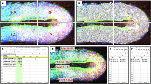
Cell segmentation for analysis and finding PSM-somite border

(A) Split image into four images using “Crop 3D”. One of the her1^ci301;her7^hu2526 mutant embryos is used as a repesentative sample.

(B) Segmented cells are seen in the Right-Anterior, Right-Posterior, Left-Anterior, and Left-Posterior of the tissue.

(C) An example of XLS file, which includes statistics of “Cell Number of Vesicles”, “Cell Position”, and “Cell Volume”.

(D) Measurement points for anterior PSM border.

(E and F) Add X and Y data of the points in the “Somite” sheet of the (E) left-anterior and (F) right-anterior XLS file.

Measuring angle of expression stripes along the posterior-anterior axis

(A–C) Measuring angle of expression stripes along the posterior-anterior axis and linear fitted equation for angle data (A), (B), and (C) show different wild-type samples as an example for measuring angle and distance of stripe to tailbud. Scale bar is 100 µm.

(D) Plot “Angle vs Distance (μm)” graph to fit an equation, where the slope and Y-intersected data provide “delta_angle” and “angle”, respectively.

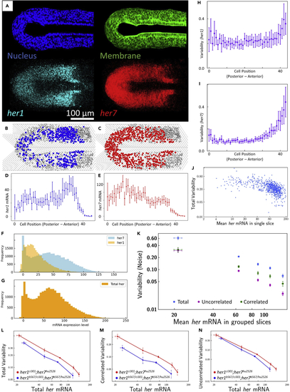
Example outcomes of images, RNA and variability (noise) distributions

(A–N) (A) Masked nucleus (blue) and membrane (green) frames, and 3D projection of her1 (cyan) and her7 (red) transcripts of a her1^ci301;her7^hu2526 mutant embryo. Scale bar is 100 µm. (B) and (C) show heatmaps of cells containing her1 (blue) and her7 (red) that are higher than an arbitrary threshold in single-cell-wide slices, respectively. (D) and (E) show her1 (blue) and her7 (red) RNA distribution along the posterior-anterior axis of the right-side of the embryo. Error bars are two standard errors of mean (SEM). (F) and (G) show the frequency histograms of her1 (transparent orange) and her7 (transparent blue), and total her (opaque orange) RNA expression per cell of her1^ci301;her7^hu2526 mutant embryos (n=17, N=2), respectively. N is the number of independent experiments; n is the number of embryos. (H) and (I) show the average transcription variabilities of her1 and her7 per slice along the posterior-anterior axis. Error bars are two SEM. (J) shows total variability of mean her RNA levels of each single slice. (K) shows average of total (blue), correlated (green), and uncorrelated (purple) variabilities versus binned mean her RNA levels of slices. Error bars are two SEM. (L), (M), and (N) show total, correlated, and uncorrelated variability plots of multiple genetic backgrounds, her1^ci301;her7^hu2526 (red, n=17, N=2) and her1^b567/ci301;her7^b567/hu2526 (blue, n=12, N=2) mutant embryos. Adapted from Zinani et al.³ N is the number of independent experiments; n is the number of embryos. Error bars are two SEM.

Comparison between “good” and “bad” fixed embryos