
|
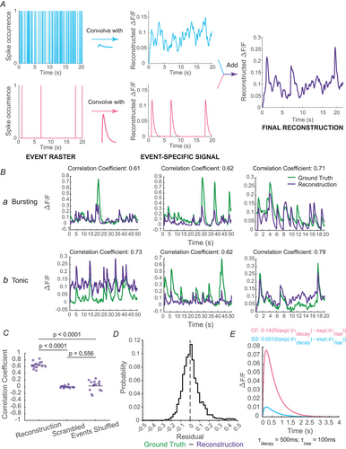
Fig. 3 RECONSTRUCTION OF THE CALCIUM SIGNAL FROM ELECTROPHYSIOLOGY TRACES A, schematic showing the method used to reconstruct the calcium signal from an electrophysiological trace. Simple spike (cyan) and CF input (magenta) rasters (left) are independently convolved with calcium sensor kernels (cyan for simple spikes, magenta for CF inputs) to generate an event-specific calcium signal time series (middle). These are then simply added together to get the final reconstruction (right). B, comparison of ground truth (green) and reconstructed (purple) calcium signals for three randomly chosen bursting cells (Ba) and three randomly chose tonic cells (Bb). The Pearson's correlation coefficient between the two traces is marked above the plot for each pair. C, correlation coefficients for all cells calculated for either the true reconstruction, a scrambled version of the reconstruction, or the reconstruction for when simple spike and CF input event times were shuffled. A Kruskal–Wallis test yielded a P value of 2.108 × 10⁻⁷, which was followed by a post hoc Dunn's test for individual comparisons, the latter of which is marked on the figure (n = 15 cells; six bursting, nine tonic). D, distribution of residuals between the ground truth and reconstructed calcium signal, pooled across all cells (n = 15 cells). E, the optimal calcium sensor kernels for simple spikes (cyan) and CF inputs (magenta). The formula for each kernel is mentioned above the plots, and the values for rise and decay time constants are mentioned below the plot.